Finite Volume Neural Network

The motivation

The picture above shows a scientist (strangely resembling Sheldon Cooper) with a robot assistant, working together to discover a useful pattern from an experiment that they just conducted. This picture is an analogy of a hybrid modeling framework, where physical knowledge (originating from the scientist's expertise) is combined with the capability to learn patterns from data (represented by the robot and its computing capability). This hybrid model, also known as the physics-informed machine learning model, has the potential to develop into a very powerful model. Unfortunately, the existing models are either too physically-rigid so that its learning ability is restricted, or too flexible so that its predictions are physically inconsistent and implausible. Additionally, they are mostly trained on synthetically-generated datasets, and rarely on real world data.

Enter the Finite Volume Neural Network (FINN)!

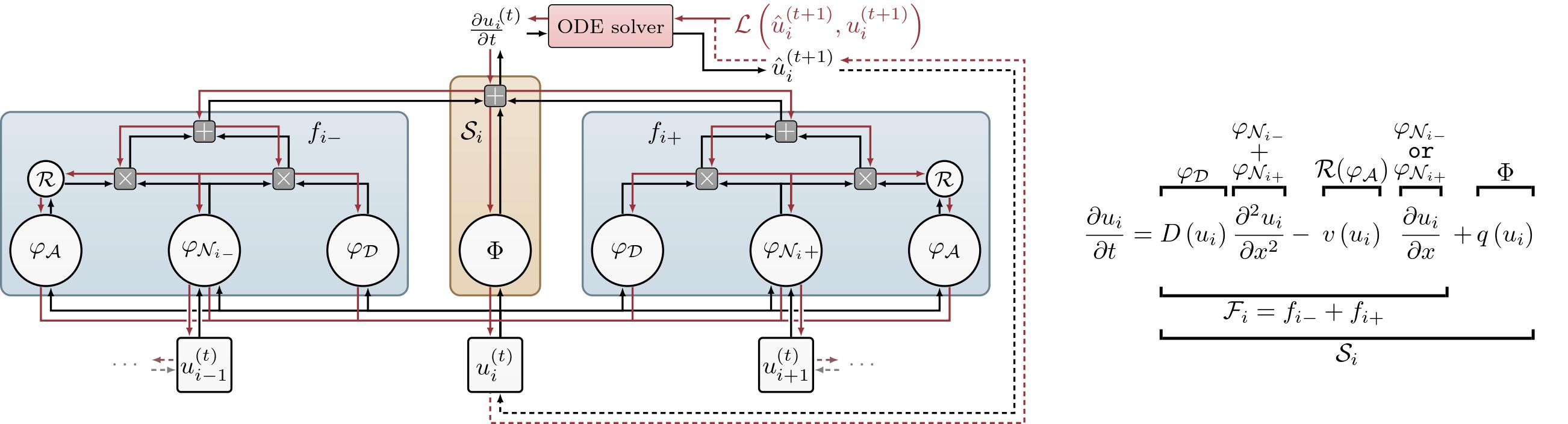
In this project, we introduce the Finite Volume Neural Network (FINN) to solve and learn unknown parts of advection-diffusion equations. As its name suggests, FINN adopts the structure of the Finite Volume Method (FVM), which is one of the most famous numerical methods for solving Partial Differential Equations (PDEs). Individual elements used in the FVM are replaced with learnable neural network modules (see the sketch below). This way, the model structure itself regularizes the model training, and we are able to learn unknown parts of the equations explicitly because it mimics the general form of the equation. The other nice thing about FINN is that it can handle different types of numerical boundary conditions, unlike models with convolutional structure.

How does FINN compare to other models?

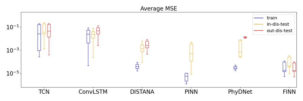
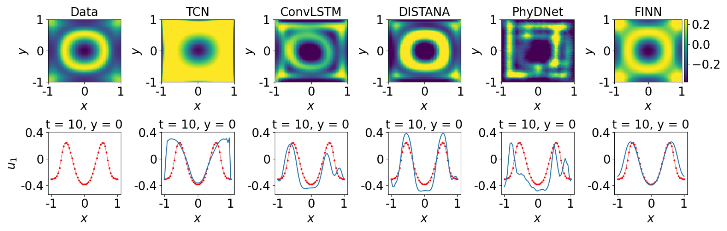
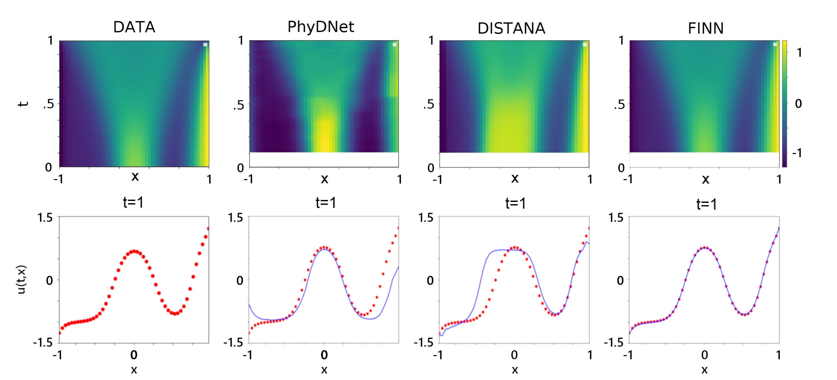
To demonstrate FINN's performance, we trained FINN and other models on synthetically generated datasets. As test datasets, we defined the in-distribution (in-dis-test) datasets as the extrapolated train datasets, and the out-of-distribution datasets (out-dis-test) that are generated with different initial or boundary conditions. The plot above shows the prediction error comparison of FINN with various deep learning models. The important point to emphasize is that FINN has favorable prediction consistency, even on out-dis-test datasets. As opposed to FINN, the other models have comparable errors during training (except for TCN and ConvLSTM), but their performance deteriorates significantly on in-dis-test, and even worse on out-dis-test data. A visualization of the out-dis-test predictions on the Fitzhugh-Nagumo diffusion-reaction equation is shown in the plot below. Qualitatively, FINN's prediction also resembles the data the most, whereas the other model predictions are quite erratic.

What about real world data?

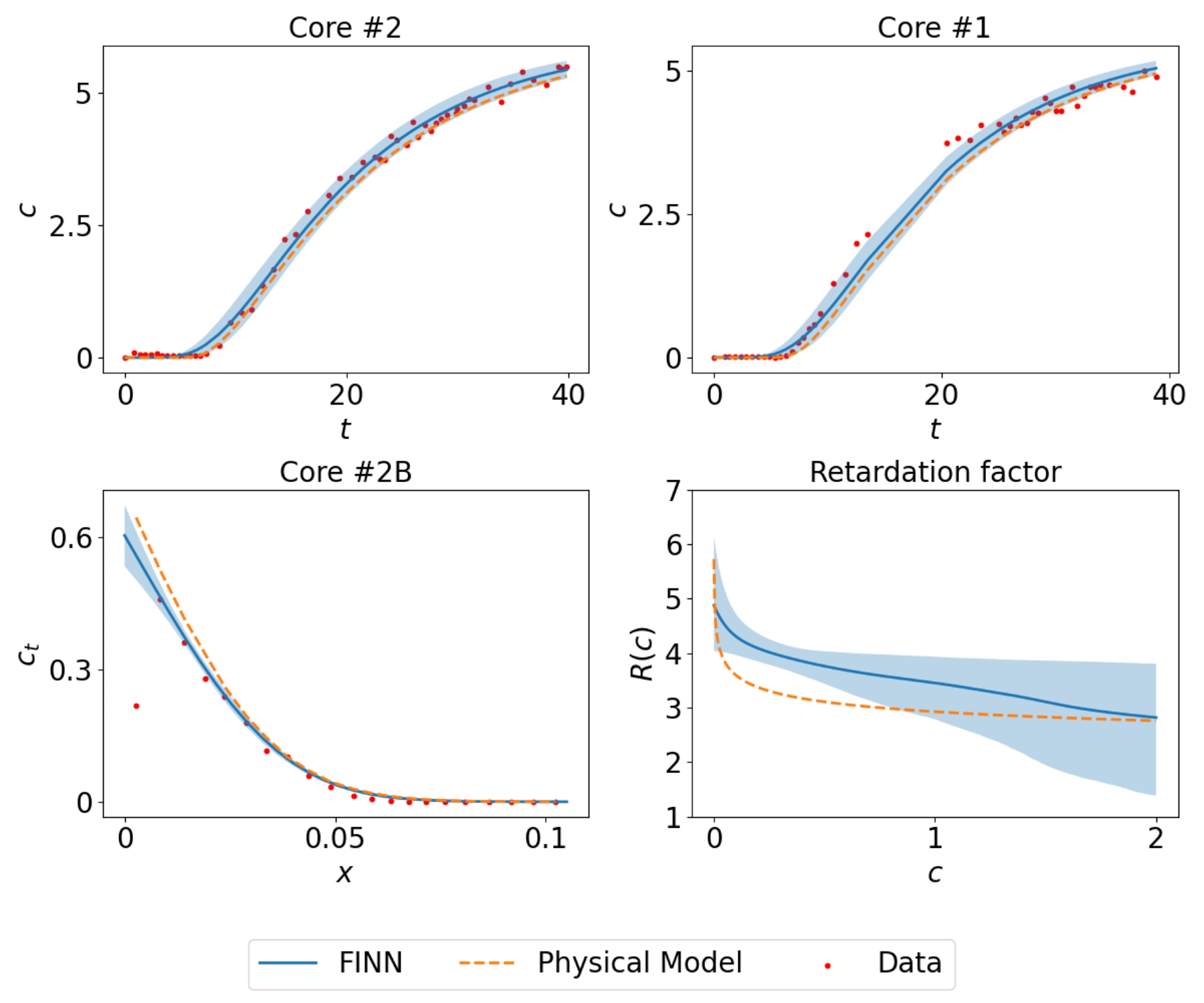
Yes, I argued earlier that other models have rarely been tested on real world data. So what happens then when FINN is trained with real and noisy datasets? As a demonstration, we employed laboratory measurement data of a groundwater contaminant diffusion through soil. Due to the limitations of the measuring equipment and the experimental design, the measured data are sparse and noisy. For training, we only used 55 data points that originated from a single core sample (core #2, top left plot in the figure below)! As expected, FINN was still able to learn the unknown closure function (the retardation factor in this particular application, bottom right plot in the figure below). This learned closure function was then used to predict the diffusion processes in other core samples (core #1 and #2B). One of these samples (#2B) has a significantly longer size, and therefore, has to be modelled with a different numerical boundary condition type. Additionally, because FINN is relatively scalable, we were able to implement the Markov Chain Monte Carlo (MCMC) algorithm to quantify the model and prediction uncertainty. In the plot below, we show ensembles of FINN's prediction. The average prediction even outperforms the calibrated physical model!

Boundary condition inference

You might have noticed that I already mentioned boundary condition several times in this article. This is simply because boundary condition is extremely important in solving PDEs. Without a well-defined boundary condition, unique solutions to PDEs do not exist. Not convinced yet? Think about a weather forecasting task. Numerical weather predictors are usually applied only on a designated location (e.g. a country, a city, or even a smaller area). However, weather from outside of this observed region also influences the processes inside the modeled area. This influence should be encoded as the boundary conditions of the modeled domain, in order to have a reliable weather prediction. This encoding process is often not very straightforward. Therefore, we also experimented on infering a yet unknown boundary condition value with FINN. Compared to the other models, FINN was again able to accurately infer the boundary condition values, resulting in higher prediction accuracy (see the plot below).

TLDR

In conclusion, we introduced FINN, which combines the structure of the Finite Volume Method (FVM) and the learning ability of ANNs. In short, elements of the FVM discretization are replaced with ANN modules. As a result, the model is interpretable and data efficient. Another important thing to note is that FINN has been successfully applied on varying or even unknown boundary conditions, and on real world data. In future works, it will be interesting to modify the implementation to facilitate applications to irregular grids and heterogeneous systems, so that it can be implemented on a larger scale (for example field scale instead of just laboratory scale experiment).